if (!require("pacman")) install.packages("pacman")# use this line for installing/loadingpacman::p_load(devtools) pacman::p_load(tidyverse, openintro, gtable, ggrepel, patchwork, units, readr, gt, gganimate, gifski, png, ggplot2, ggh4x, ggrepel, ggridges)
Abstract
The Psychometrics Analysis Project offers a diverse array of interactive Myer Brigs personality tests for fictional characters designed for personal entertainment, these tests aim to provide insights into various aspects of personality assessment It’s primary focus is on presenting the types defined by ISTJ and ENFP by understanding these personalities types individuals can gain insights into their own behaviors, preferences and interpersonal dynamics the key traits are associated with each type, emphasizing the diverse ways in which individual interact with the world based on the personality prefrences.
Introduction
This project leverages data collected by the Open-Source Pyschometrics Project to reveal the relationship between popular culture and psychology. Through non-orthodox data analysis methods, 890 characters from 100 different universes could be compared and contrasted for their personalities. Each fictional universe denotes a different tv show or movie with popular characters within. While the characters used are fictional, the methods produced by this project will be re-usable and, in theory, applicable to collections of real-world people.
Question 1:
How do Myers-Briggs personality types distribute across different universes, and how does the average match percentage vary within each universe? Additionally, is there any correlation between character notability scores and their Myers-Briggs types within each universe?
Introduction
Question one is primarily an exploration of the varying personality types that exist across cultural media. It looks to investigate the differences in character personalities and motivations across differing universes, potentially identifying correlations between genres or settings. Additionally, an attempt to uncover a relationship between popular opinion of characters and their in-universe personas will be made: are anti-heroes liked more? Are villains viewed more negatively than heroes? These questions will be answered providing information about the prevalence and celebration of particular personality types, which enhance our comprehension of audience engagement and storytelling dynamics.
Approach
Initially the dataset was loaded from the “TidyTuesday” source using the read.csv function in R. The date and location columns were verified to ensure that they are in the correct data types. The dataset containing information about characters is where the Data Collected to visualise various universes and their personality traits from the Open Psychometrics Project website (or you can provide the link), By exploring the data and examining the structure of the dataset to understand its variables and general content. This includes inspecting the Characters, Psychology Stats, and Myers-Briggs tables which performs preprocessing of any necessary data steps, such as handling missing values, data type conversion, and cleaning up variable names Moreover, one of it could be exploring data analysis, distribution of character notability scores across different universes, inquire the distribution of personality traits among characters, including the most common traits and any notable patterns or trends analyzing the average ratings and standard deviations of personality traits to understand the variability within each trait, Exploring the distribution of Myers-Briggs personality types across characters and universes examining the percentage match of Myers-Briggs types and the number of user respondents for each character. To create visualizations to represent key findings from the exploring of data analysis. This could include bar plots, scatter plots, and radar plots to visualize distributions, correlations, and patterns with the notability scores for different types of Myer Briggs personality type, Through interpretation of statistical analysis tests to determine if there are momentous differences in character notability scores between universes there have been some statistical tests conducted to determine each character notability scores and personaltiy traits for Myers-Briggs types.
Analysis
Code
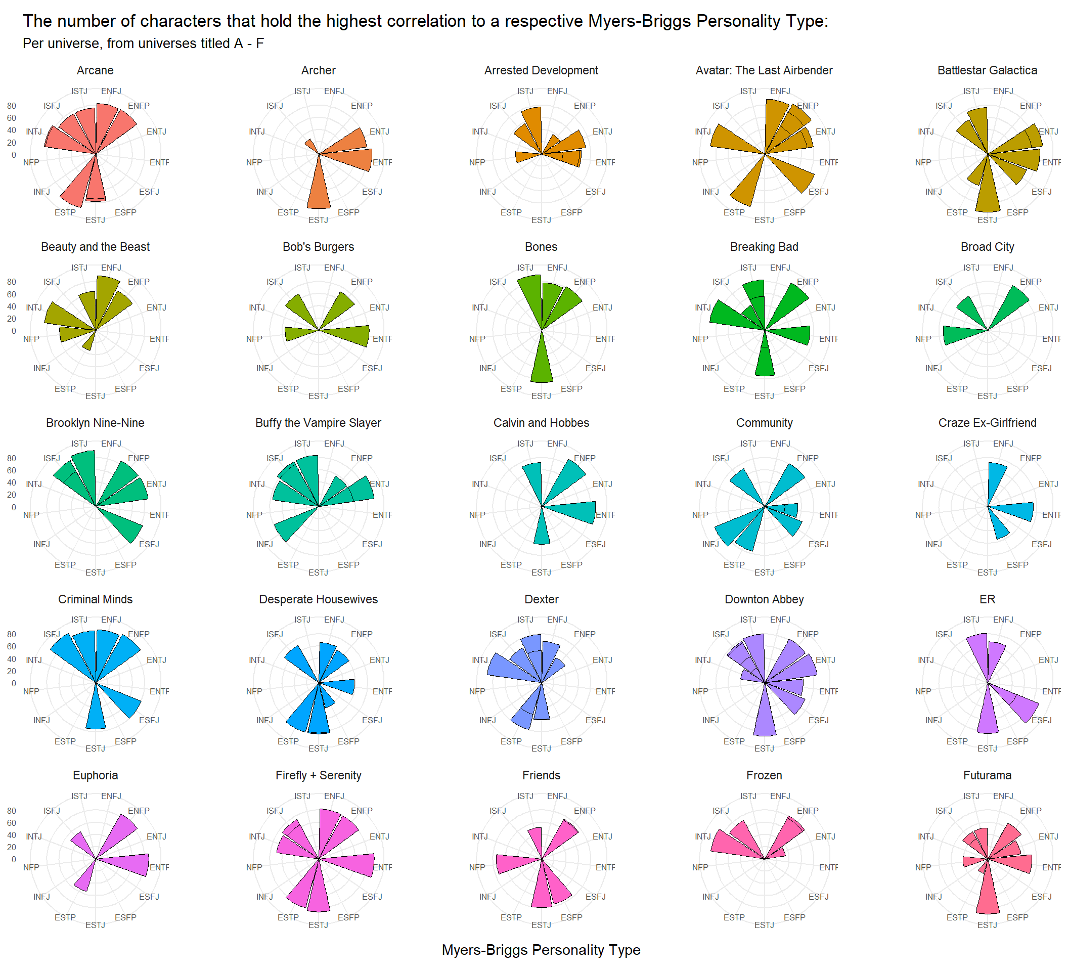
#plotA <- ggplot(data = myers_briggs) + geom_density(aes( group = uni_name, x = avg_match_perc, ))#plotA#unique(myers_briggs$uni_name)pacman::p_load(viridis, RColorBrewer)pacman::p_load(magick, nflplotR)pacman::p_load(RColorBrewer)#FUNCTION TO TAKE ATTRIBUTE THE PERSONALITY TYPE OF EACH CHARACTER BASED ON WHICH THEY MATCH WITH THE MOSTmyers_briggs_grouped <- myers_briggs %>%group_by(char_name) %>%#summarise(max = max(avg_match_perc, na.rm=TRUE))slice_max(avg_match_perc)# introverted versus extroverted; sensing versus intuitive; thinking versus feeling; and perceiving versus judging.#SUB GROUPING OF DATA BY ADDING TWO NEW COLUMNS FOR SOCIALISATION AND HOW THEY PERCEIVE THE WORLDmyers_briggs_grouped <- myers_briggs_grouped %>%mutate(socialisation =case_when(substr(myers_briggs, 1, 1) =="E"~"Extroverted",substr(myers_briggs, 1, 1) =="I"~"Introverted" ),empiricism =case_when(substr(myers_briggs, 2, 2) =="N"~"Intuitive",substr(myers_briggs, 2, 2) =="S"~"Sensing" ) )#LINKING OF THE MYERS_BRIGGS.CSV AND CHARACTERS.CSV TO JOIN PERSONALITY TYPES AND NOTABILITY SCORES - THEN ARRANGED BY UNIVERSE NAME IN ALPHABETICAL ORDERmyers_briggs_linked <-left_join(myers_briggs_grouped, characters, by=c("char_name"="name", "char_id"="id", "uni_id"="uni_id", "uni_name"="uni_name"))myers_briggs_linked <- myers_briggs_linked %>%arrange(by = uni_name)#FOUR UNIVERSE PLOTS TO MAP THE 99 UNIVERSES COUNTS OF CHARACTERS OF GIVEN PERSONALITY TYPES#EACH PLOT TAKES A SUBSECTION OF THE ALPHABETICALLY-ORDERED UNIVERSES AND APPLIES THE FOLLOWING ELEMENTS#CREATES A RADIAL COLUMN PLOT OF MYERS-BRIGGS AGAINST NOTABILITY, FACET WRAPPED BY UNIVERSE NAMEmyersBriggsUniversePlot1 <-ggplot(myers_briggs_linked[starts_with(LETTERS[1:6], vars=myers_briggs_linked$uni_name),]) +theme_minimal() +geom_col(aes(x = myers_briggs, y = notability, fill = uni_name), size=.05, color="black", position=position_dodge()) +theme(axis.title.y =element_blank(), axis.text =element_text(size =6), panel.grid.minor=element_blank(), title =element_text(size =11), plot.subtitle =element_text(size =10), plot.background =element_rect(color ="white"), legend.text =element_blank(), legend.position ="none", panel.spacing.x =unit(4, "lines"), strip.clip ="off") +scale_y_continuous(breaks = scales::breaks_width(20)) +labs(title ="The number of characters that hold the highest correlation to a respective Myers-Briggs Personality Type: ", subtitle="Per universe, from universes titled A - F", x ="Myers-Briggs Personality Type") +coord_polar() +facet_wrap2(vars(uni_name))myersBriggsUniversePlot2 <-ggplot(myers_briggs_linked[starts_with(LETTERS[7:13], vars=myers_briggs_linked$uni_name),]) +theme_minimal() +geom_col(aes(x = myers_briggs, y = notability, fill = uni_name), size = .05, color ="black", position =position_dodge()) +theme(axis.title.y =element_blank(), axis.text =element_text(size =6), panel.grid.minor=element_blank(), title =element_text(size=11), plot.subtitle =element_text(size =10), plot.background =element_rect(color ="white"), legend.text =element_blank(), legend.position ="none", panel.spacing.x =unit(4, "lines"), strip.clip ="off") +scale_y_continuous(breaks = scales::breaks_width(20)) +labs(title="The number of characters that hold the highest correlation to a respective Myers-Briggs Personality Type: ", subtitle="Per universe, from universes titled G - M") +coord_polar() +facet_wrap2(vars(uni_name))myersBriggsUniversePlot3 <-ggplot(myers_briggs_linked[starts_with(LETTERS[14:19], vars=myers_briggs_linked$uni_name),]) +theme_minimal() +geom_col(aes(x = myers_briggs, y = notability, fill = uni_name), size=.05, color="black", position=position_dodge()) +theme(axis.title.y =element_blank(), axis.text =element_text(size =6), panel.grid.minor =element_blank(), title =element_text(size=11), plot.subtitle =element_text(size=10), plot.background =element_rect(color ="white"), legend.text =element_blank(), legend.position ="none", panel.spacing.x =unit(4, "lines"), strip.clip ="off") +scale_y_continuous(breaks = scales::breaks_width(20)) +labs(title="The number of characters that hold the highest correlation to a respective Myers-Briggs Personality Type: ", subtitle="Per universe, from universes titled N - S") +coord_polar() +facet_wrap2(vars(uni_name))myersBriggsUniversePlot4 <-ggplot(myers_briggs_linked[starts_with(LETTERS[20:26], vars = myers_briggs_linked$uni_name),]) +theme_minimal() +geom_col(aes(x = myers_briggs, y = notability, fill = uni_name), size = .05, color ="black", position=position_dodge()) +theme(axis.title.y =element_blank(), axis.text =element_text(size =6), panel.grid.minor =element_blank(), title =element_text(size =11), plot.subtitle =element_text(size =10), plot.background =element_rect(color ="white"), legend.text =element_blank(), legend.position ="none", panel.spacing.x =unit(4, "lines"), strip.clip ="off") +scale_y_continuous(breaks = scales::breaks_width(20)) +labs(title ="The number of characters that hold the highest correlation to a respective Myers-Briggs Personality Type: ", subtitle="Per universe, from universes titled T - Z") +coord_polar() +facet_wrap2(vars(uni_name))#THE FOLLOWING PLOTS OF QUESTION ONE USE VARIOUS COLOUR PALETTES FROM THE RCOLORBREWER PACKAGE#THIS PLOT FOLLOWS THE SAME FORMAT AS THE PREVIOUS FOUR, BUT DOES NOT DISSECT BASED ON ALPHABETICAL SEQUENCE, AND INSTEAD IS BASED ON FOUR GIVEN UNIVERSES: THE WALKING DEAD, GAME OF THRONES, FRIENDS AND BROOKLYN NINE-NINE - TO SEE HOW THEY COMPARE AND CONTRASTmyersBriggsUniversePlotZoomed <-ggplot(myers_briggs_linked[myers_briggs_linked$uni_name %in%c("Brooklyn Nine-Nine", "Friends", "Game of Thrones", "The Walking Dead"),]) +geom_col(aes(x = myers_briggs, y = notability, fill = uni_name), size=.05, color="black", position=position_dodge()) +theme_minimal() +theme(axis.title.y =element_blank(), axis.text =element_text(size =10), panel.grid.minor =element_blank(), title =element_text(size=15), plot.subtitle =element_text(size =10), plot.background =element_rect(color ="white"), legend.text =element_blank(), legend.position ="none", panel.spacing.x =unit(4, "lines"), strip.clip ="off") +scale_y_continuous(breaks = scales::breaks_width(20)) +labs(title="The number of characters that hold the highest correlation to\na respective Myers-Briggs Personality Type: ", subtitle ="For four universes", x ="Myers-Briggs Personality Type") +coord_polar() +facet_wrap2(vars(uni_name)) +scale_fill_brewer("PRGn")#THEGGSAVE PACKAGE IS EMPLOYED TO SAVE THE BROKEN DOWN UNIVERSE PLOTS AS IMAGES, TO ALLOW FOR EASIER RESIZINGggsave("images/universePlot.png", myersBriggsUniversePlot1, width =20, height =15, units =c("in"))ggsave("images/universePlot2.png", myersBriggsUniversePlot2, width =20, height =15, units =c("in"))ggsave("images/universePlot3.png", myersBriggsUniversePlot3, width =20, height =15, units =c("in"))ggsave("images/universePlot4.png", myersBriggsUniversePlot4, width =20, height =15, units =c("in"))myersBriggsUniversePlot1
Code
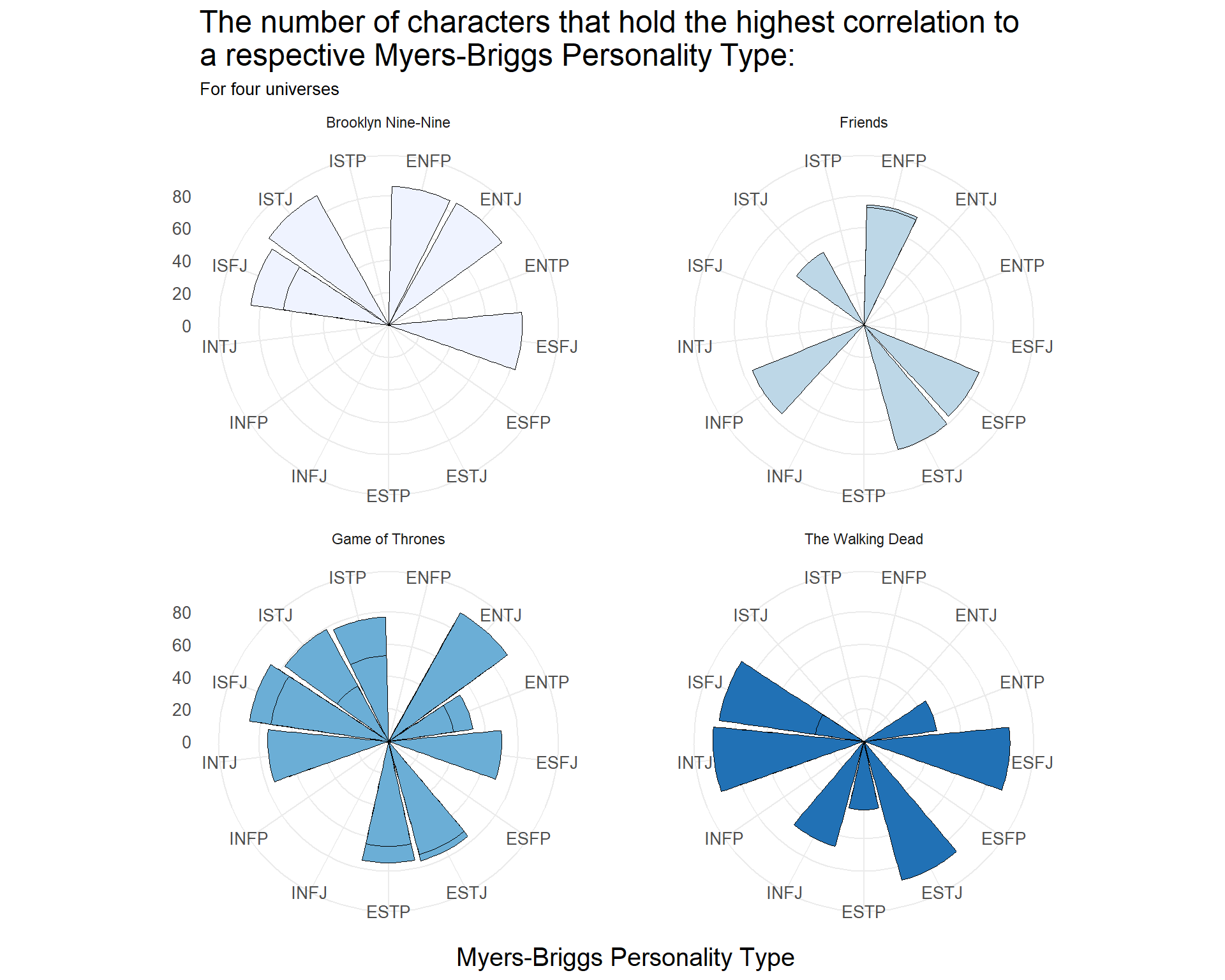
#GGSAVE IS USED TO SAVE THE UNIVERSE PLOT OF THE FOUR-SELECTED-SHOWS, TO ALLOW FOR EASIER RESIZINGggsave("images/universePlot5.png", myersBriggsUniversePlotZoomed, width =20, height =10, units =c("in"))myersBriggsUniversePlotZoomed
Code
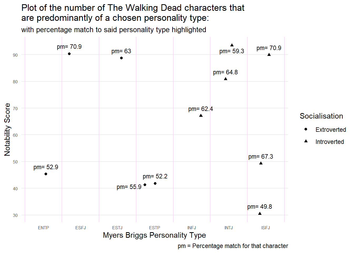
#THE FOLLOWING FOUR PLOTS ALTERNATE IN TWOS: THE FIRST AND THIRD OF THE FOUR DEAL WITH INDIVIDUAL CHARACTER NOTABILITY SCORES, WHILE TWO AND FOUR DEAL WITH THEIR MEANED AVERAGES#PLOTS ONE AND THREE (CONCERNING THE WALKING DEAD AND GAME OF THRONES, RESPECTIVELY) BOTH USE THE SAME APPROACH - A GEOM JITTER PLOT THAT PLACES THE INDIVIDUAL CHARACTERS WITHIN THEIR DOMINANT PERSONALITY TYPE, WITH THE Y-AXIS REPRESENTING THEIR NOTABILITY TO THE AUDIENCE#ABOVE EACH CHARACTERS POINT IS THEIR PERCENTAGE MATCH WITH THEIR ASSIGNED DOMINANT PERSONALITY TRAIT, TO SHOW THAT MOST CHRACTERS DO NOT EASILY FIT JUST ONE PERSONALITY CATEGORY#THE VISUALISATION LAYOUT IS: A GEOM JITTER | A BLANK THEME | GEOM REPELLED TEXT (TO ENSURE TEXT LABELS DONT OVERLAP) | VERTICAL LINES TO SEPARATE THE PERSONALITY TYPES#PLOTS TWO AND FOUR TAKE THE AVERAGED MEANS OF NOTABILITY FOR THEIR ENTIRE PERSONALITY TYPES AND VISUALISE THESE VALUES - ALLOWING FOR AN AVERAGED UNDERSTANDING OF WHICH CHARACTERS TYPES ARE MORE NOTABLE WITHIN CERTAIN GENRES OF MEDIA#THE VISUALISATION LAYOUT IS: A GEOM BARPLOT USING STATISTICAL MEAN | A BLANK THEME | GEOM TEXT | VERTICAL LINES TO SEPARATE THE PERSONALITY TYPES#THE WALKING DEADnotabilityScores_TheWalkingDead <-ggplot(myers_briggs_linked[myers_briggs_linked$uni_name %in%c("The Walking Dead"),], aes()) +theme_minimal() +geom_jitter(aes(x = myers_briggs, y = notability, pch = socialisation), position =position_jitter(seed=3)) +theme(plot.background =element_rect(color ="white"), axis.text =element_text(size=6), panel.grid.minor.y=element_blank(), title =element_text(size =11), plot.subtitle =element_text(size=10), axis.text.x =element_text(), panel.grid.major.x =element_blank()) +scale_y_continuous(breaks = scales::breaks_width(10)) +labs(title="Plot of the number of The Walking Dead characters that\nare predominantly of a chosen personality type: ", subtitle="with percentage match to said personality type highlighted", x ="Myers Briggs Personality Type", y ="Notability Score", caption="pm = Percentage match for that character", pch ="Socialisation") +geom_text_repel( aes( label =paste("pm=",avg_match_perc), x = myers_briggs, y = notability), size=3, vjust=-1, position =position_jitter(seed =3)) +geom_vline(xintercept =seq(0.5, after_stat(nrow(myers_briggs)),1), color="#FFAAFF", alpha = .5)notabilityScores_TheWalkingDead
Code
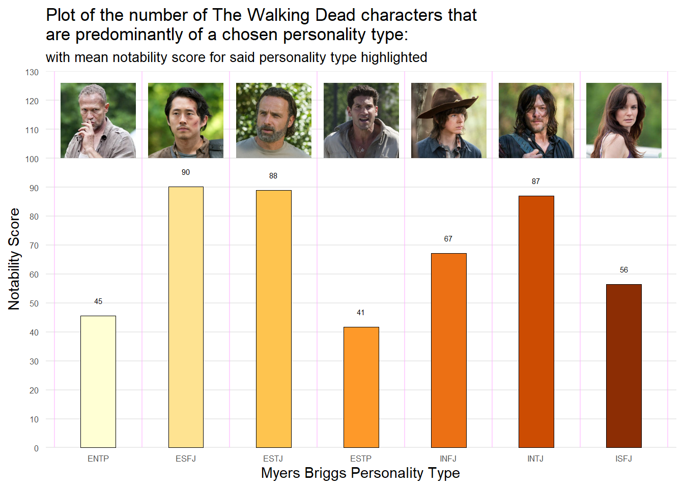
notabilityMeans_TheWalkingDead <-ggplot(filter(myers_briggs_linked, uni_name =="The Walking Dead"), aes(group = myers_briggs, x = myers_briggs)) +theme_minimal() +geom_bar(aes( y = notability, fill = myers_briggs), width=.4, stat="summary", fun="mean", colour="black", size =0.2) +theme(plot.background =element_rect(color ="white"), panel.grid.minor.y=element_blank(), title =element_text(size=11), plot.subtitle =element_text(size=10), axis.text =element_text(size=6), panel.grid.major.x =element_blank(), legend.position ="none") +scale_y_continuous(breaks = scales::breaks_width(10), expand =expand_scale(c(0,0), c(0,35))) +labs(title="Plot of the number of The Walking Dead characters that\nare predominantly of a chosen personality type: ", subtitle="with mean notability score for said personality type highlighted", x ="Myers Briggs Personality Type", y ="Notability Score") +geom_vline(xintercept=seq(0.5,after_stat(nrow(myers_briggs)),1),color="#FFAAFF", alpha = .5) +stat_summary(geom="text", fun ="mean", aes(label=floor(after_stat(y)), x = myers_briggs, y = notability), size =2, vjust=-2) +geom_from_path(aes(x = myers_briggs, y=95, path = image_link, group=myers_briggs), width = .2, height = .2, vjust=-.2) +scale_fill_brewer(palette ="YlOrBr")notabilityMeans_TheWalkingDead
Code
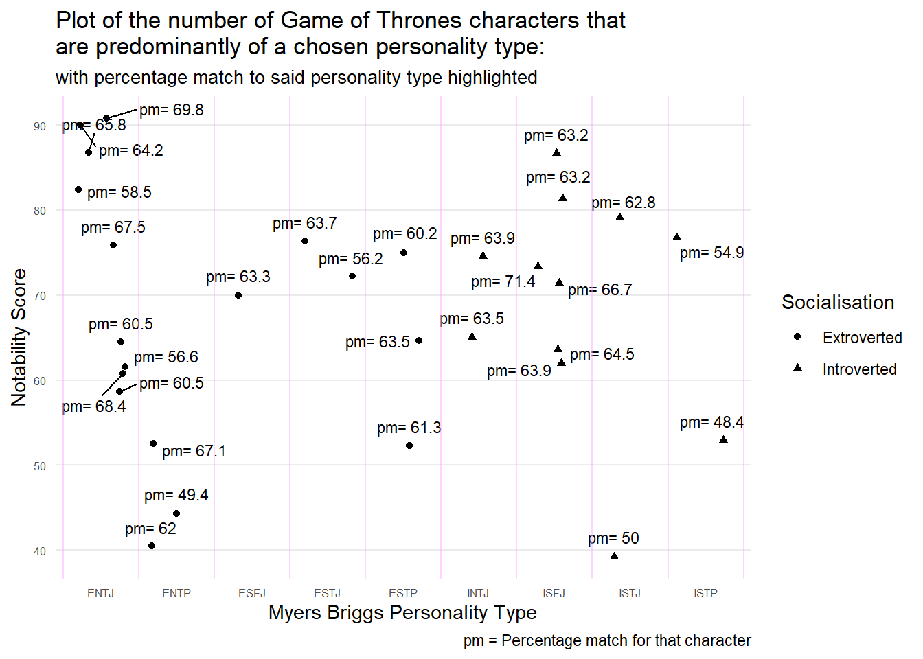
#GAME OF THRONESnotabilityScores_GameOfThrones <-ggplot(myers_briggs_linked[myers_briggs_linked$uni_name %in%c("Game of Thrones"),], aes()) +theme_minimal() +geom_jitter(aes(x = myers_briggs, y = notability, pch=socialisation), position =position_jitter(seed=3)) +theme(plot.background =element_rect(color ="white"), axis.text =element_text(size=6), panel.grid.minor.y=element_blank(), title =element_text(size=11), plot.subtitle =element_text(size=10), axis.text.x =element_text(), panel.grid.major.x =element_blank()) +scale_y_continuous(breaks = scales::breaks_width(10)) +labs(title="Plot of the number of Game of Thrones characters that\nare predominantly of a chosen personality type: ", subtitle="with percentage match to said personality type highlighted", x ="Myers Briggs Personality Type", y ="Notability Score", caption="pm = Percentage match for that character", pch ="Socialisation") +geom_text_repel( aes( label=paste("pm=",avg_match_perc), x = myers_briggs, y = notability), size=3, vjust=-1, position =position_jitter(seed=3)) +geom_vline(xintercept=seq(0.5,after_stat(nrow(myers_briggs)),1),color="#FFAAFF", alpha = .5)notabilityScores_GameOfThrones
Code
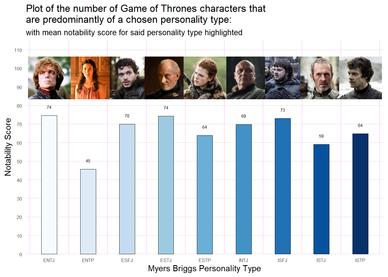
notabilityMeans_GameOfThrones<-ggplot(filter(myers_briggs_linked, uni_name =="Game of Thrones"), aes(group = myers_briggs, x = myers_briggs)) +geom_bar(aes( y = notability, fill = myers_briggs), width=.4, stat="summary", fun="mean", colour="black", size =0.2) +theme_minimal() +theme(plot.background =element_rect(color ="white"), panel.grid.minor.y=element_blank(), title =element_text(size=11), plot.subtitle =element_text(size=10), axis.text =element_text(size=6), panel.grid.major.x =element_blank(), legend.position ="none") +scale_y_continuous(breaks = scales::breaks_width(10), expand =expand_scale(c(0,0), c(0,20))) +labs(title="Plot of the number of Game of Thrones characters that\nare predominantly of a chosen personality type: ", subtitle="with mean notability score for said personality type highlighted", x ="Myers Briggs Personality Type", y ="Notability Score") +geom_vline(xintercept=seq(0.5,after_stat(nrow(myers_briggs)),1),color="#FFAAFF", alpha = .5) +stat_summary(geom="text", fun ="mean", aes(label=floor(after_stat(y)), x = myers_briggs, y = notability), size =2, vjust=-2) +geom_from_path(aes(x = myers_briggs, y=95, path = image_link, group=myers_briggs), width = .2, height = .2) +scale_fill_brewer(palette ="Blues")notabilityMeans_GameOfThrones
Code
#GGSAVE TO PRODUCE IMAGES OF THE FOUR PLOTS FOR RESIZINGggsave("data/notabilityScores_TheWalkingDead.png", notabilityScores_TheWalkingDead, width =9, height =5, units =c("in"))ggsave("data/notabilityMeans_TheWalkingDead.png", notabilityMeans_TheWalkingDead, width =9, height =5, units =c("in"))ggsave("data/notabilityScores_GameOfThrones.png", notabilityScores_GameOfThrones,width =9, height =5, units =c("in"))ggsave("data/notabilityMeans_GameOfThrones.png", notabilityMeans_GameOfThrones, width =9, height =5, units =c("in"))
Code
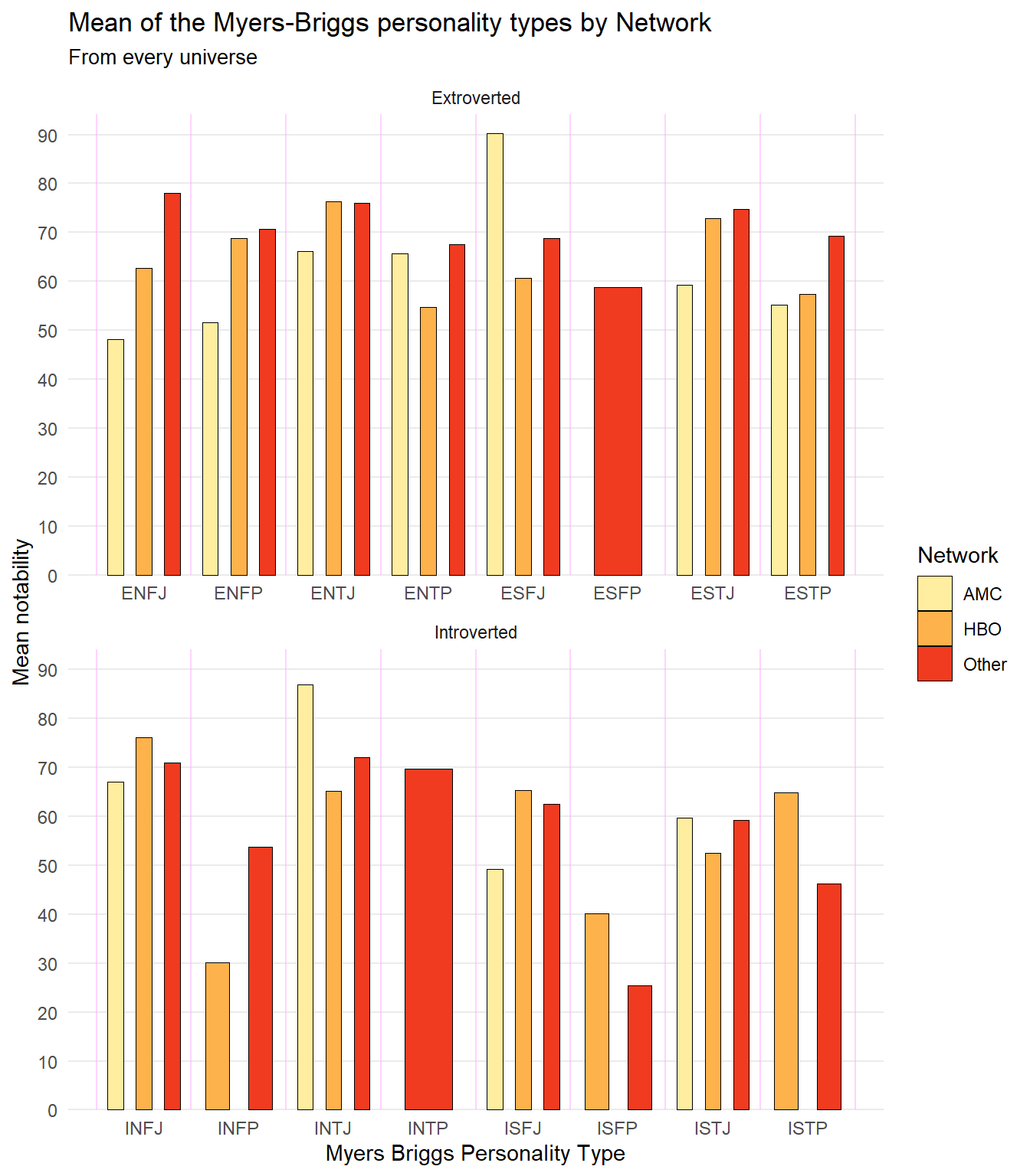
#CODE USED TO TEST THE VIABILITY OF GROUPING MEAN NOTABILITY VALUESmyers_briggs_mean_notability <- myers_briggs_linked %>%group_by(uni_name, myers_briggs) %>%summarise(mean =mean(notability),socialisation = socialisation,empiricism = empiricism ) %>%filter(mean ==max(mean))#g11 <- ggplot(myers_briggs_mean_notability) + geom_bar(aes(x = myers_briggs, fill = myers_briggs)) + theme( panel.grid.minor.y=element_blank(), title = element_text(size=11), plot.subtitle = element_text(size=10), axis.text = element_text(size=6), panel.grid.major.x = element_blank(), legend.position = "none") + scale_y_continuous(breaks = scales::breaks_width(2), expand = expand_scale(c(0,0), c(0,4))) + labs(title="Count of the myers-briggs type correlated to the highest mean notability scores", subtitle="From every universe", x = "Myers Briggs Personality Type", y = "Count") + geom_text( aes( label=after_stat(count), x = myers_briggs, y = after_stat(count)), vjust=-1, size = 3, stat="count")#g11#CODE USED TO TEST THE VIABILITY OF GROUPING MEAN NOTABILITY VALUESmyers_briggs_mean_notability <- myers_briggs_mean_notability %>%mutate(Network =case_when( uni_name %in%c("Game of Thrones", "True Detective", "Euphoria", "The Sopranos", "Westworld", "The Wire", "Watchmen", "Succession", "Silicon Valley") ~"HBO", uni_name %in%c("Breaking Bad", "Better Call Saul", "Mad Men", "The Walking Dead", "") ~"AMC",TRUE~"Other" ))#THE MEAN NOTABILITY SCORES OF EACH PERSONALITY TYPE, FOR EVERY UNIVERSE ARE MAPPED TO A NEW DATASET, ALONGSIDE THEIR SOCIALISATION AND PERCEPTION TYPESmyers_briggs_grouped_notability <- myers_briggs_linked %>%group_by(uni_name, myers_briggs) %>%summarise(notability = (notability),socialisation = socialisation,empiricism = empiricism )#MEDIA NETWORKS OF HBO AND AMC ARE ADDED TO INCLUDE THEIR MOST POPULAR SHOWS WITHIN THE DATASET, VIA APPENDING THE NEW DATASETmyers_briggs_grouped_notability <- myers_briggs_grouped_notability %>%mutate(Network =case_when( uni_name %in%c("Game of Thrones", "True Detective", "Euphoria", "The Sopranos", "Westworld", "The Wire", "Watchmen", "Succession", "Silicon Valley") ~"HBO", uni_name %in%c("Breaking Bad", "Better Call Saul", "Mad Men", "The Walking Dead") ~"AMC",TRUE~"Other" ))#THE MEAN NOTABILITY PER NETWORK FOR EACH PERSONALITY TYPE IS VISUALISED VIA A BAR PLOT THAT HAS A MAXIMUM OF THREE BARS PER PERSONALITY TYPE FOR HBO, AMC AND ALL OTHER NETWORKS - THIS IS THEN SAVED AS AN IMAGE VIA GGSAVEperNetwork_MeanNotability <-ggplot(myers_briggs_grouped_notability) +geom_bar(aes(x = myers_briggs, fill = Network, y = notability), stat="summary", fun ="mean", position =position_dodge(.9), width = .5, colour="black", size =0.2) +theme_minimal() +theme(plot.background =element_rect(color ="white"), panel.grid.minor.y=element_blank(), title =element_text(size=11), plot.subtitle =element_text(size=10), axis.text =element_text(size=9), panel.grid.major.x =element_blank(), ) +scale_y_continuous(breaks = scales::breaks_width(10), expand =expand_scale(c(0,0), c(0,4))) +labs(title="Mean of the Myers-Briggs personality types by Network", subtitle="From every universe", x ="Myers Briggs Personality Type", y ="Mean notability") +facet_wrap2(vars(socialisation), scales ="free_x", nrow =2) +scale_fill_brewer(palette ="YlOrRd") +scale_x_discrete(expand=(c(.1,.1))) +geom_vline(xintercept=seq(0.5,after_stat(nrow(myers_briggs)),1),color="#FFAAFF", alpha = .5) perNetwork_MeanNotability
Code
ggsave("images/perNetwork_MeanNotability.png", perNetwork_MeanNotability, width =8, height =7, units =c("in")) #END
Discussion
A multiplicity of insights can be garnered from the multitude of graphs displayed while evaluating the myer-briggs personality types of various characters across media. To begin, a wide variation exists between almost every television show and film included within the data, showcasing that some universes hold more introverted characters, some more judging, some more perceptive and so on. While the data is far from exhaustive of all popular television, these insights did allow for further srutiny and comparison - such as recognising that Game of Thrones actually contains a large number of introverted characters, potentially attributed to its setting in the medieval period.
Similarly, a closer inspection of The Walking Dead and Game of Thrones yielded interesting results. Based on the percentage match scores, which determine how close a character fitted their predominant personality type, it can be discerned that no one character held a strong enough percentage match average to declare that they held one, strict personality type: although some were close (above 70% percentage match average). In continuation, the mean notability scores yielded knowledge on which personalities resonated more with audiences in certain settings. The Walking Dead’s dystopian society may have had an impact on the popularity of ESFJ, ESTJ and INTJ types:
ESFJ or Consuls, who are extremely social, generous and reliable
ESTJ or Executives, who are diplomatic in nature and are diligent and efficient
INTJ or Architects, who are complicated, introverts with high intellects that are straight-forward and rationale
On the other hand, Game of Thrones’ characterisations have yet to reveal drastic differences between character notability. This may reveal hidden factors that affect an audience’s perception of characters and thus, their perceived noteworthiness.
Finally, the mean notability of characters divided by network allows one to make a number of potential conclusions. From the data alone, AMC is better at producing Judging characters, while HBO and AMC have yet to create characters that fit every major personality type available.
What is the frequency distribution of character personality traits across all characters, and how does it correlate with their average rating? Furthermore, do character notability scores vary significantly based on their personality traits?
Introduction
Intriguing insights into the dynamics of character perception and storytelling impact can be gained by examining the frequency distribution of personality qualities in characters and how they relate to average ratings. One could explore whether a character that is commonly perceived as honourable or righteous has a resonance with the audience, or even a more fulfilling character arc. Tying this to the real-world it could be utilised to determine whether traits such as lazy correlate to a lesser perception of an individual from their peers.
Approach
To address these problems comprehensively, we will conduct a multifaceted analysis of the Psychometrics Project dataset. Initially, we will scrutinize the frequency distribution of character personality traits across the entire dataset. This examination will involve quantifying the occurrence of each personality trait and visualizing the distribution using appropriate graphical representations, such as bar charts or radar charts.Subsequently, we will delve into exploring the correlation between character personality traits and their average ratings. This analytical pursuit necessitates calculating the correlation coefficient to ascertain the degree of association between personality trait scores and average ratings. Visualization techniques, such as scatter plots coupled with regression analysis, will aid in elucidating the nature and strength of this correlation, we will investigate the potential variability of character notability scores contingent upon their respective personality traits. Employing statistical methodologies( write what methods did you use)Moreover, we will assess whether there exist significant differences in notability scores across distinct personality trait categories. Visual aids such as density plots and bar plots will complement this analysis, providing clear illustrations of any discernible variations in notability scores among different personality trait cohorts. By meticulously examining these facets of the dataset, we aim to derive profound insights into the interplay between character personality traits, average ratings, and notability scores. Such insights hold the dynamics underlying character portrayal and reception within the dataset, thereby contributing to a deeper understanding of human behavior and perception in the context of fictional character depiction.
Analysis
Code
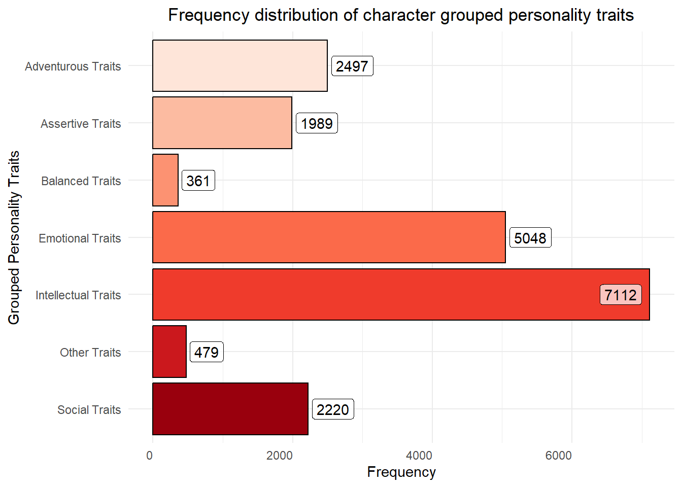
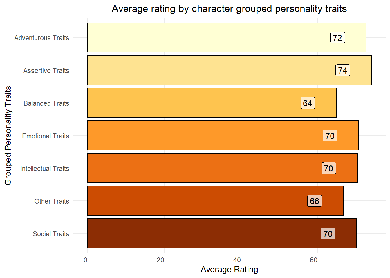
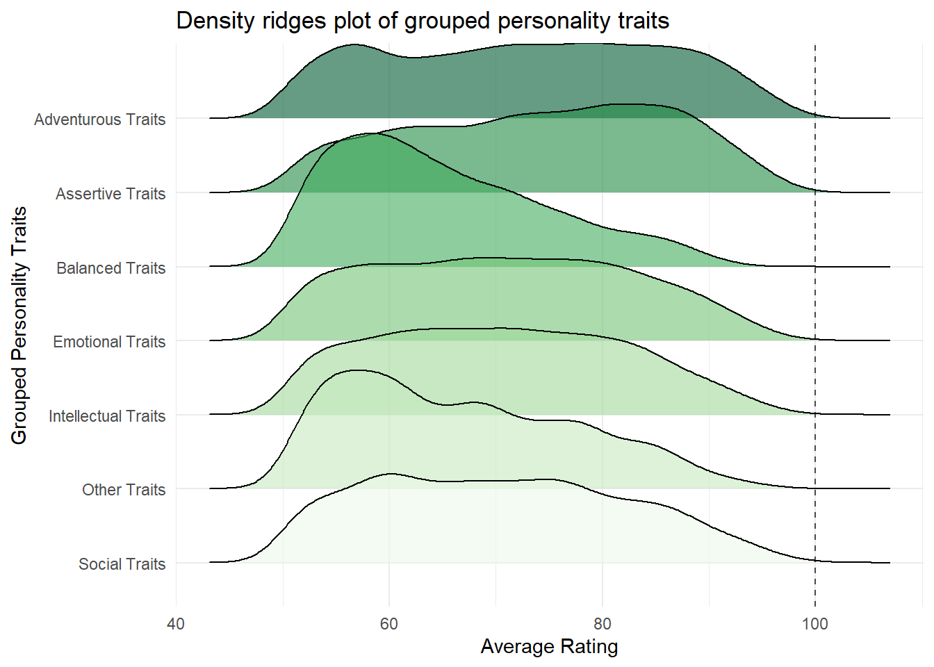
characters$char_id = characters$idpsych_stats$personality_category <-sapply(psych_stats$personality, categorize_personality)personalityDistribution <- psych_stats |>count(personality_category)personalityDistribution =subset(personalityDistribution, personality_category !="Unknown")charactersFiltered = characters |>select(char_id, notability)psychStatsFiltered = psych_stats |>select(char_id, personality_category, avg_rating)psychStatsCharacters =merge(charactersFiltered, psychStatsFiltered, by ="char_id")psychStatsCharactersSubset =subset(psychStatsCharacters, personality_category !="Unknown")avgRating = psychStatsCharacters |>group_by(personality_category) |>summarise(avg_rating =mean(avg_rating))avgNotability = psychStatsCharacters |>group_by(personality_category) |>summarise(avg_notability =mean(notability))psychStatsCharactersMerged =merge(personalityDistribution, avgRating, by ="personality_category")psychStatsCharactersMerged =merge(psychStatsCharactersMerged, avgNotability,by ="personality_category")personalityDistribution =subset(personalityDistribution, personality_category !="Unknown")avgRating =subset(avgRating, personality_category !="Unknown")avgNotability =subset(avgNotability, personality_category !="Unknown")question2Part1Plot1 =ggplot(personalityDistribution, aes(x =factor(fct_rev(fct_inorder(personality_category))), y = n)) +geom_bar(stat ="identity", aes(fill=(personality_category)), color ="black") +scale_fill_brewer(palette ="Reds") +labs(title ="Frequency distribution of character grouped personality traits",x ="Grouped Personality Traits",y ="Frequency") +coord_flip() +theme_minimal()+theme(axis.text.x =element_text( hjust =1),plot.title =element_text(hjust =0.5), legend.position ="none", plot.background =element_rect(color ="white")) +geom_label(aes(x = (factor(fct_rev(fct_inorder(personality_category)))), y = n, label=floor(n), hjust =ifelse(personality_category =="Intellectual Traits", 1.2, -.1)), color ="black", alpha =0.7)question2Part1Plot2 =ggplot(avgRating, aes(x =factor(fct_rev(fct_inorder( personality_category))), y = avg_rating)) +geom_bar(stat ="identity", aes(fill = (personality_category)), color ="black") +labs(title ="Average rating by character grouped personality traits",x ="Grouped Personality Traits",y ="Average Rating") +coord_flip() +theme_minimal() +scale_fill_brewer(palette ="YlOrBr")+theme(axis.text.x =element_text(hjust =1),plot.title =element_text(hjust =0.5), legend.position ="none", plot.background =element_rect(color ="white")) +geom_label(aes(x = (factor(fct_rev(fct_inorder( personality_category)))), y = avg_rating, label =floor(avg_rating)), hjust =2.5, color ="black", alpha =0.7)question2Part2Plot =ggplot(avgNotability, aes(x =factor(fct_rev(fct_inorder( personality_category))), y = avg_notability)) +geom_bar(stat ="identity", aes(fill= (personality_category)), color ="black") +labs(title ="Average notability by character grouped personality traits",x ="Grouped Personality Traits",y ="Average Notability") +coord_flip() +theme_minimal() +scale_fill_brewer(palette ="Purples")+theme(axis.text.x =element_text( hjust =1),plot.title =element_text(hjust =0.5), legend.position ="none", plot.background =element_rect(color ="white")) +geom_label(aes(x = (factor(fct_rev(fct_inorder(personality_category)))), y = avg_notability, label =floor(avg_notability)), hjust =2.5, color ="black", alpha =0.7)question2Part1Plot3 =ggplot(psychStatsCharactersSubset, aes(x = avg_rating, y =factor(fct_rev(personality_category)))) +geom_density_ridges(aes(fill =factor(fct_rev( personality_category))), alpha =0.6) +theme_minimal() +theme(legend.position ="none", plot.background =element_rect(color ="white")) +labs(title="Density ridges plot of grouped personality traits", x ="Average Rating", y ="Grouped Personality Traits") +scale_fill_brewer(palette ="Greens") +geom_vline(xintercept =100, color ="black", alpha =0.7, linetype ="dashed")# old plot q2p2oldPlot =ggplot(psychStatsCharactersSubset, aes(x = avg_rating)) +geom_density(aes(fill = personality_category), alpha = .7) +facet_wrap(~personality_category, dir ="v") +theme_minimal() +scale_fill_brewer(palette ="Greens") +scale_y_continuous(breaks =seq(0,0.04, 0.04)) +theme(legend.position ="none", axis.text.x=element_text(angle =c(45,rep(0,4),45))) +labs(title="Density plot of grouped personality traits", x="Average Rating", y="Density")# saving the plots in pngggsave("images/question2Part1Plot1.png", question2Part1Plot1, width =9, height =5, units =c("in"))ggsave("images/question2Part1Plot2.png", question2Part1Plot2, width =9, height =5, units =c("in"))ggsave("images/question2Part1Plot3.png", question2Part1Plot3, width =9, height =5, units =c("in"))ggsave("images/question2Part2Plot1.png", question2Part2Plot, width =9, height =5, units =c("in"))question2Part1Plot1
Code
question2Part1Plot2
Code
question2Part1Plot3
Code
question2Part2Plot
Discussion
Conclusion:
To sum up, the examination of Myers-Briggs personality types in different universes shows some interesting trends. Every universe displays a distinct distribution of personality types, indicating possible associations with media genres or topics. For example, whilst “Downton Abbey” features more outgoing characters, “Buffy the Vampire Slayer” tends to include more reclusive ones. This finding raises more questions about how preferences for storytelling could affect the characteristics of characters across genres.
Furthermore, there is no discernible relationship between the average rating and the frequency distribution of character personality traits across all worlds. Characters generally obtain average ratings that are comparable regardless of their personality type. This implies that other elements, such as plot, character development, and acting ability, may have a greater impact on audience reaction than certain personality qualities.
Moreover, there is little variation in character notability scores according to personality factors. The data shows that the average notability scores of the various personality categories don’t differ all that much. This suggests that a character’s relevance and impact within their own universe might have less to do with their personality attributes and more to do with how they are portrayed, role-played, and given weight in the story.
In general, personality types and qualities seem to have less of an impact on audience perception and character notability than other aspects, even though they may add to the diversity and complexity of characters in different media universes. This emphasizes how difficult it is to develop characters and hold an audience’s interest in pop culture and entertainment.